Rise of the Modern AI Empire – The Transformer

The article explains the working of the Transformer with a step-by-step explanation.

The list of content is given below:

• Introduction
• Why Transformer?
• Transformer Overview
• The Engine Behind Foundation Models (The Transformer)
• Training Vs Inference
• Some Applications
• Conclusion

I. INTRODUCTION

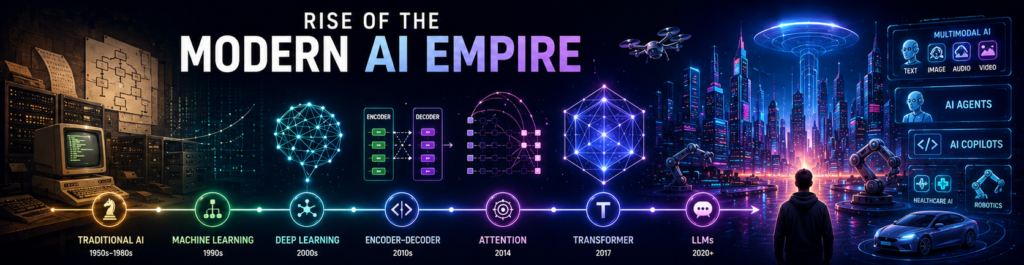
After the 1950s, Artificial Intelligence (AI) evolved very fast. With a clear understanding of Mathematics, programming, and critical thinking, researchers and scientists started to dig deeper and deeper, and then ML was introduced. ML enables computational systems to learn patterns or relationships from data and use them to make predictions, decisions, and give outputs without explicit human help. With the rapid advancements of Machine Learning (ML), the landscape of AI started to change to something more beautiful.

Neural Network research had existed for decades, but during the 2000s, advances in data, computational power, optimization, etc. helped establish what we now call Deep Learning (DL). In DL, neural networks get deeper, meaning the number of layers is much larger. And it becomes more powerful. However, since 70s to 2012, there were many algorithms and architectures that could do very amazing tasks; since 2012, DL has become more popular, and we know this year as the Big Bang of Deep Learning.

Although DL evolves very fast, there is still something that cannot be solved with its former algorithms, such as long–context representation. Then, in 2017, an architecture was introduced to the world based on the encoder-decoder architecture. The architecture was named “The Transformer” in the paper, “Attention Is All You Need”. This architecture has the working idea of an encoder-decoder, but the difference is the attention mechanism. Yes, the attention mechanism was introduced in 2014, but the attention mechanisms in the Transformer are self-attention, multi-head attention, masked multi-head attention, and cross-attention mechanisms.

The Transformer was proposed as an alternative to recurrent and convolutional sequence-transduction architectures, particularly for machine translation. Its key innovation was replacing recurrence/convolution in the sequence-processing architecture with attention mechanisms. But with the idea behind it, there are many organizations, people, and institutions who have worked and are working to introduce a lot of new architectures. So, the Transformer subsequently became the architectural foundation for many influential model families. Different models adopted different parts of the Transformer: BERT uses an encoder-only design, and GPT uses a decoder-only design. These Transformer-based models eventually developed into what are now commonly called foundation models.

II. WHY TRANSFORMER?

In sequential processing like Machine Translation, the architectures Recurrent Neural Networks can perform a good task. When they are in the encoder-decoder architecture, they handle the process very well and handle the translation very well. But they produce a fixed-size vector even when we have a very long sentence that is to be translated. So, it becomes a problem because it doesn’t have contextual meaning. These architectures process the input sequence one token at a time, meaning one word is processed and then another word. This becomes a very headache-inducing and long process. These two are the main problems that the Transformer is here to solve.

III. TRANSFORMER OVERVIEW

Why do we call this architecture the Transformer? The answer is simple, and you will get the understanding of this answer when you read this section and the next section.

“We call this architecture the Transformer because it completely transforms an input sequence into an output sequence using a stack of attention mechanisms”. So, it’s similar to the Transformers in the movie Transformers. In the movie, the cars are completely transformed into robots. Cars are the input sequence, and robots are the output sequence. Think of the Transformer architecture like this.

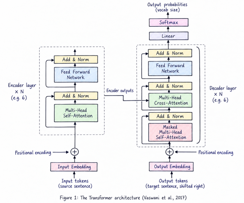
Transformer has both an encoder and a decoder. It is based on the encoder-decoder idea. So, in the previous articles, we’ve discussed the encoder-decoder. Briefly, the encoder-decoder is a DL architecture that can process a sequence of input representations and produce a sequence of output representations.

In the encoder, the transformer has 6 layers, which we know as encoder layers or encoder blocks. In each layer, there are multi-head self-attention, a residual connection and layer normalization, a position-wise Feed Forward Network, and then a second residual connection and layer normalization. And on the decoder side, there are also 6 identical layers, and we call each one of them a decoder layer or decoder block. Each layer has masked multi-head self-attention, multi-head cross-attention, a residual connection and layer normalization, and a position-wise Feed-Forward Network.

The input is tokenized and assigned token IDs. Then the IDs are converted into embeddings, and the encoder layer doesn’t know the position of the token, so we add positional encoding to tell the layer the token positions. The embedding and positional encoding both enter the multi-head self-attention layer to compute attention. And the former input, and with the output from the multi-head self-attention, they enter the Add and Normalization component. Then the output from this layer, it enters the Feed Forward Network. Then the output from this network and the output from the former Add and Normalization component enter another Add and Layer Normalization component. This is just for one layer in the encoder. The encoder has 6 layers, and this whole process is done 6 times, and then the final output is fed to the decoder.

The decoder receives the output embeddings (target word embeddings) but shifted right and with positional encoding. This input to the decoder enters the masked multi-head attention component. The output from this component and the input to the decoder enter the Add and Normalization component. The output from this and the final output from the encoder both enter an attention component, multi-head attention or the cross-attention component. The output from this enters another Add and Normalization component and then a Feed Forward Network. Then the output from the Feed Forward Network and the output from the previous Add and Normalization component enter another Add and Normalization component. This repeats 6 times because the decoder also has 6 layers. The final output is linearly projected to the vocabulary, and then the logits are fed to softmax to get real probabilities.

NB: A detailed explanation is given in the section below.

IV. The Engine Behind Foundation Models (The Transformer)

Encoder

On the encoder side, the transformer takes the entire source sequence and transforms each token into a representation that contains information about the token itself and its relationships with the other tokens. This is called contextual information.

For example, there is a sentence: “The bird can fly, and it can also sit on a tree branch”. The word ‘it’ refers to the ‘bird’ in the sentence. So, the representation of ‘it’ should contain information about itself and the surrounding tokens. Meaning, the representation should have the information that can capture relationships between ‘it’ and ‘bird’.

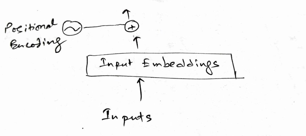
Fig. 2: Encoder Part – 1.

Before entering the transformer, the source sentence is tokenized. Tokenization is a method in which the sentence or corpus is broken down into its smallest units; in this case, the source sequence is broken down into words: word tokenization.

For example, X = “I love NLP”; X is the input. Then tokenization is X = [“I”, “love”, “NLP”].

However, each word (token) cannot be fed into the transformer architecture or any neural network. So, each token receives an integer: the token ID. Like, “I” -> 5. But this number or ID is not meaningful because it is just an index assigned to the tokens in the vocabulary.

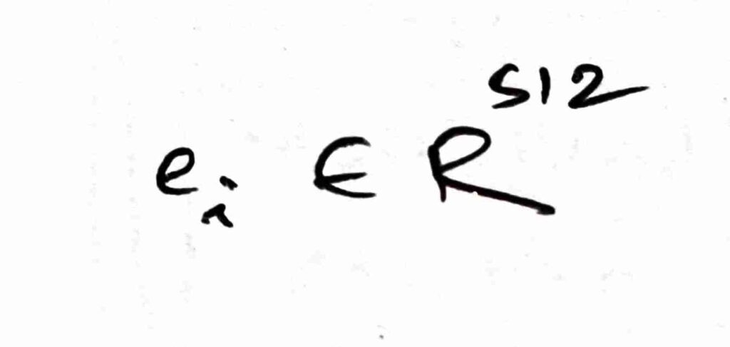
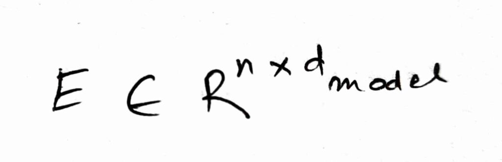
Then, the token IDs are converted into word/token embeddings. Say the vocabulary contains 40000 tokens or words; V = 40000. The transformer (the original one from the paper) uses 512 dimensions, i.e., d_model = 512; each token’s vector contains 512 numerical values.

Mathematically, every token becomes a 512-dimensional vector:

So, the embedding matrix of the whole sentence becomes:

There is another problem. The architecture doesn’t know the tokens’ positions, but for self-attention, position is very important. So, in the original Transformer, positional encoding is used.

The positional encoding (PE) used here in the original Transformer is the deterministic sinusoidal positional encoding. So, for a position pos and dimension i:

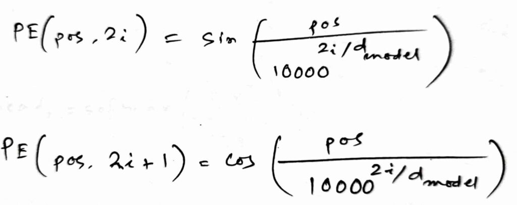
The positional encoding has the same dimension as that of the embeddings. Here, in the PE formula, inside the sin and cos functions, 10000 is a constant used by the authors, and the others are given above.

Then, the token embeddings and the positional encoding are added to get the input representation.

So, input representation = token embeddings + positional encoding.

We are going to discuss the encoder layer in detail. The input representation enters the first encoder layer (the whole encoder has 6 layers). The input goes through the multi-head self-attention mechanism.

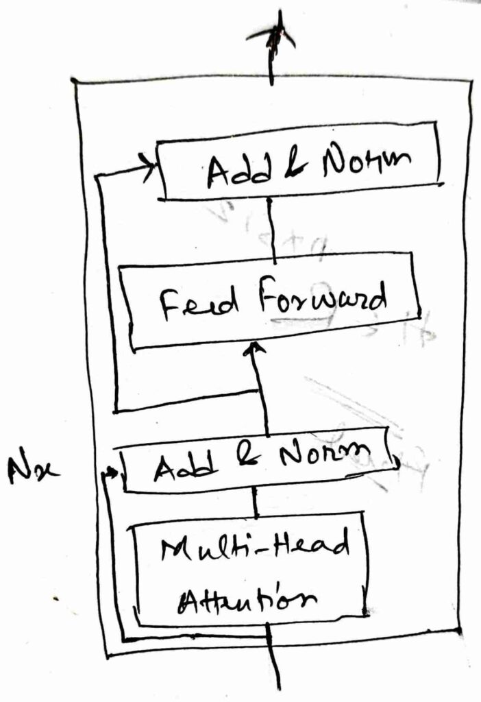
Fig. 3: Encoder part-2

The central mechanism of the Transformer architecture is the attention mechanism, and it is given by a scaled dot-product as:

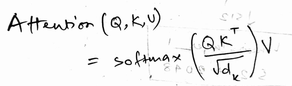
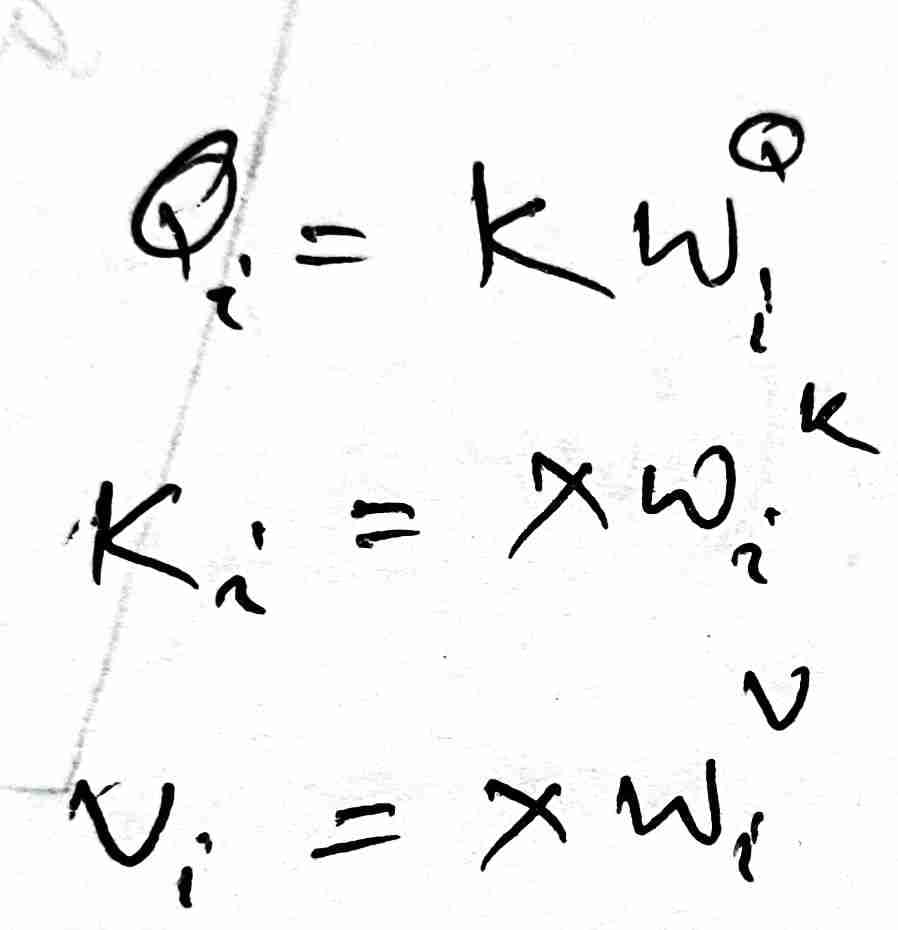
Where Q = query, K = key, and V = value are of the same dimension as the input sequence. And Q = XW^Q, K = XW^K, and V = XW^V, and

The attention calculates QK^T, so we obtain:

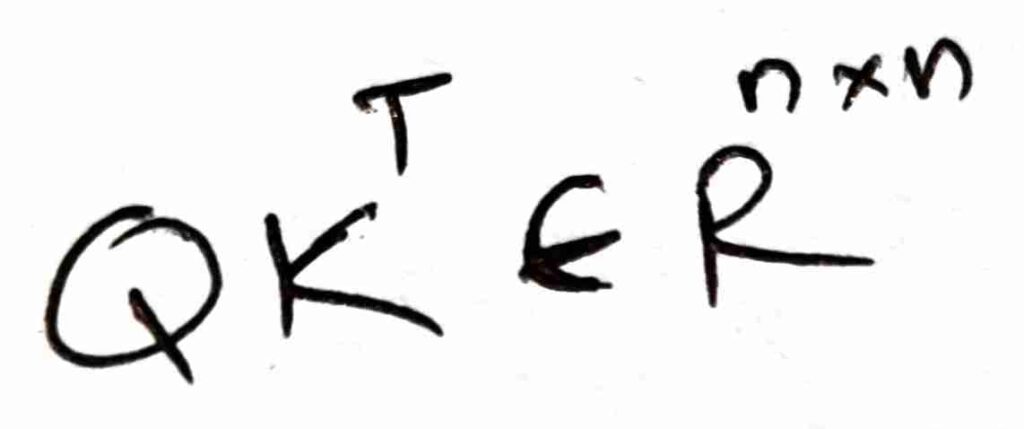
The elements in the dot product measure how strongly query i relates to key j. So each token can calculate its relationship with every token in the sequence. This is why it is called self-attention.

In the attention formula, we divide the dot product by sq. rt. d_k. This is because we need to scale the product and control the magnitude. Therefore, S = QK^T/sq. rt. d_k. Then, A = softmax(S), and the final output, O = AV. This is just for one head or one attention.

The Transformer doesn’t use one attention layer or head; it uses 8 heads; h = 8. The model dimension, d_model = 512. Each head operates with dimensions d_k = d_v = 64; then h x 64 = 512. So, instead of calculating one 512-dimensional attention space, the model learns eight different projections. 

For head i,

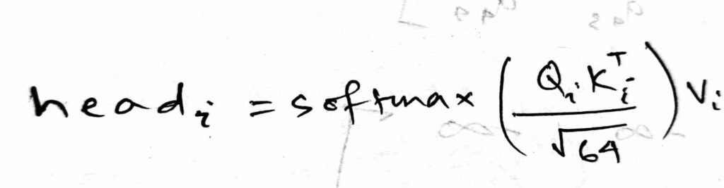
The eight outputs are concatenated as shown below.

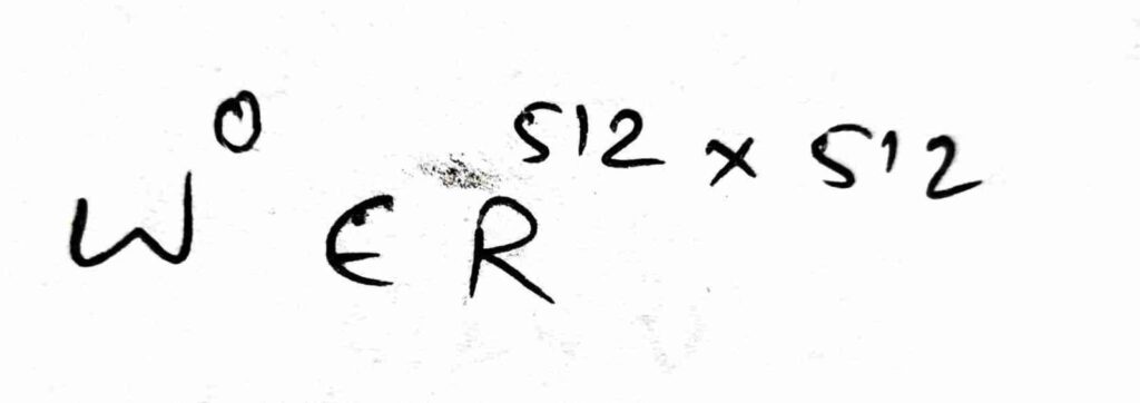
Then, Multi-head Attention = HW^O, where W^O is given below. And each head has its own W^Q, W^K, and W^V.

After multi-head self-attention, the Transformer applies a residual connection and layer normalization. The residual connection is the addition of input X with the output of multi-head attention; X + MultiHead(X, X, X).

So, for the self-attention sublayer in the paper, Z₁ = LayerNorm(X + MultiHead(X, X, X)) means: Q = X, K = X, and V = X. After the addition, normalization is performed in the original Transformer.

After this, the output is fed to position-wise Feed-Forward Network to process and transform each token’s representation independently.

FFN(x) = max(0, xW₁ + b₁)W₂ + b₂. This is because, after attention, the information is mixed, meaning the tokens are mixed, and a non-linear transformation is used here: ReLU.

The position-wise FFN is a two-layer fully connected network. The model dimension is d_model = 512; the hidden dimension of the FFN becomes d_ff = 2048. Therefore, W¹ and W² are given below.

For each token vector x:

            x -> xW₁ + b₁ -> ReLU -> (.)W₂ + b₂.

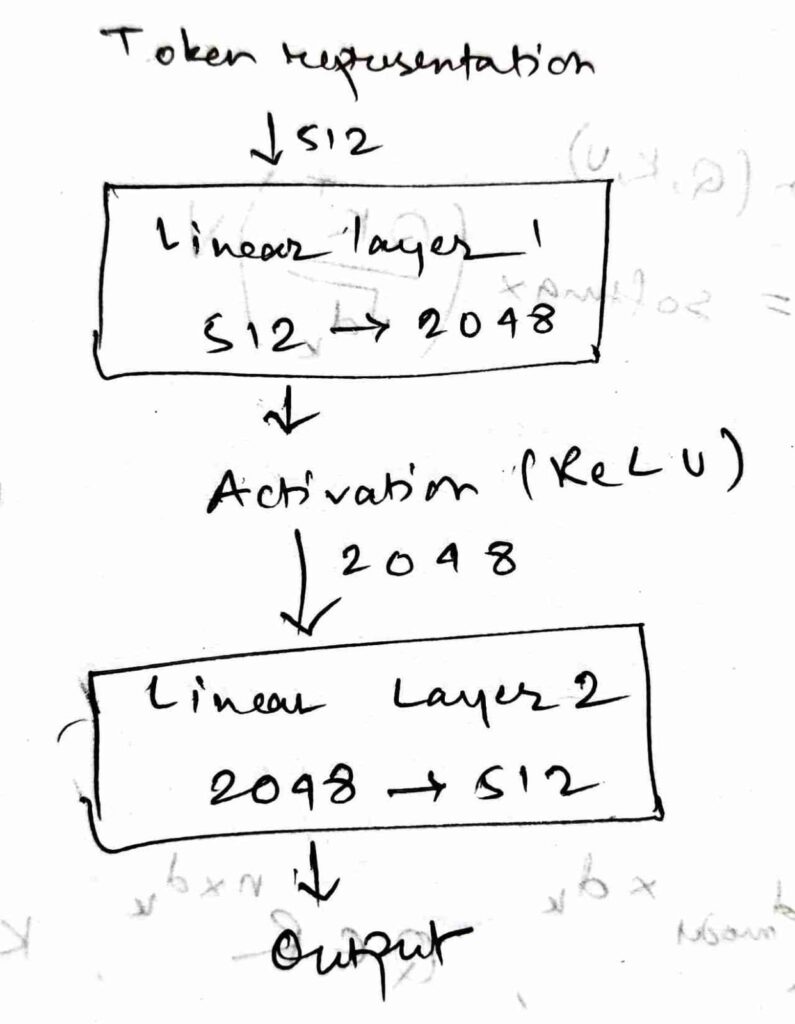
Fig. 4: Encoder part – 3

If the sequence has n tokens, the operation is effectively: FFN(x₁), FFN(x₂), …, FFN(x_n).

Again, after the FFN, there is another Add and Norm layer: a residual connection. So,

Z₂ = LayerNorm(Z₁ + FFN(Z₁)).

The complete process of one encoder layer can be summarized as: Z₁ = LN( X + MHA(X, X, X) and Z₂ = LN(Z₁ + FFN(Z₁)). The original Transformer has 6 encoder layers so; O_l = EncoderLayer(O^(l-1)), where l = 1, … , 6.

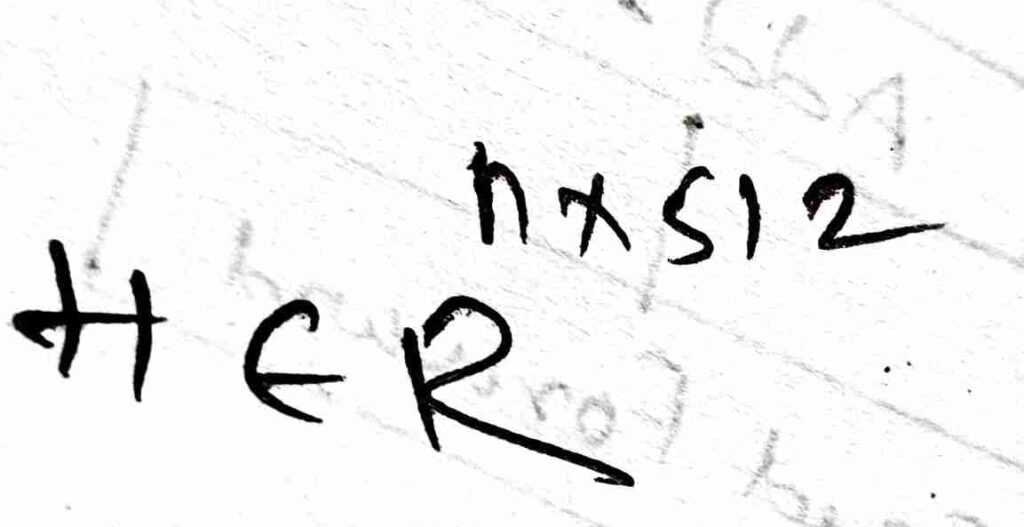
Finally, we can write the final encoder output as: H = O⁽⁶⁾, where:

Decoder

In the decoder part, the most important components are masked self-attention and cross-attention. Before we dive into the decoder, I want you to know that we use only the encoder when we want a good embedding, like BERT; meaning, if we want an understanding of the context and if we want only to generate outputs or text, we use only the decoder part like GPT, because the decoder is always autoregressive.

The input to the decoder is right-shifted with <BOS>, <START>, etc., and the process of tokenization, embedding, and positional encoding is the same as that of the encoder, so we decided to leave the explanation and continue to masked multi-head attention.

NB: <BOS> is <Beginning Of Sequence>.

NB: During training, the target sequence is shifted right and supplied to the decoder. Thus, at each position, the decoder receives the ground-truth previous target tokens rather than its own previous predictions. This training procedure is known as teacher forcing. The look-ahead mask simultaneously prevents a position from accessing future target tokens.

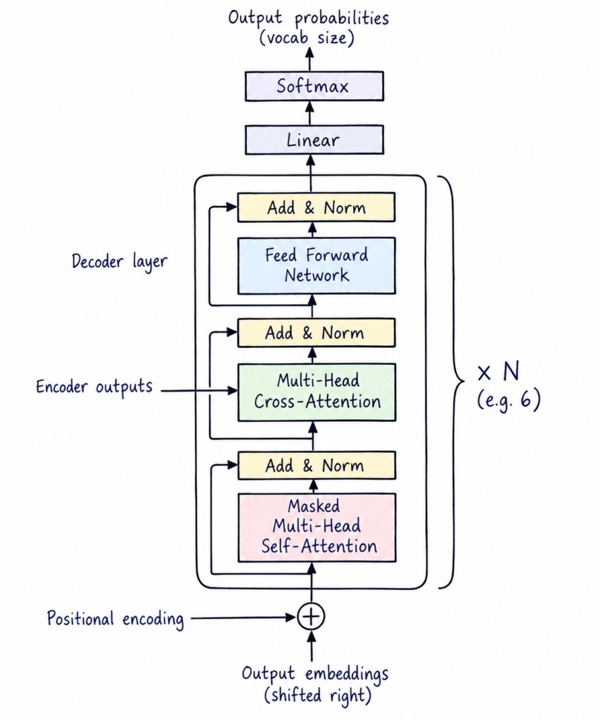
Fig. 5: Decoder

Masked Multi-Head Attention

The masked multi-head attention is one of the most important differences between the encoder and decoder. Say the target sequence is [y1,y2,y3] to predict. But when predicting y2, the decoder must not see y3. Another example: let’s say ‘I love you’ is the target sequence. During feeding to the decoder, the sentence becomes <BOS>, I, love, you. And it needs to predict I love you <EOS> (End Of Sequence). When predicting ‘love’, the decoder is allowed to use <BOS> and I but not ‘you’. But if we let the decoder know what’s coming next, the training objective would become invalid for autoregressive generation of the decoder.

So, without masking, the attention matrix can be:

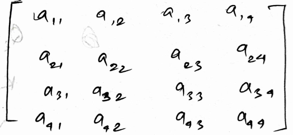
But the decoder should only attend to the current and previous positions, so the attention matrix is given as follows.

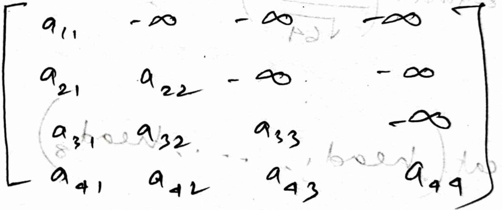
For the future positions, the decoder receives negative infinity before softmax because their attention probabilities become zero.

The masked multi-head attention is similar to the multi-head self-attention in the encoder, but the only difference is that in the decoder’s case, there is another matrix called mask, M (it is given below).

If D is the decoder’s input, then

            Q = DW^Q, K = DW^K, V = DW^V, then S is given below.

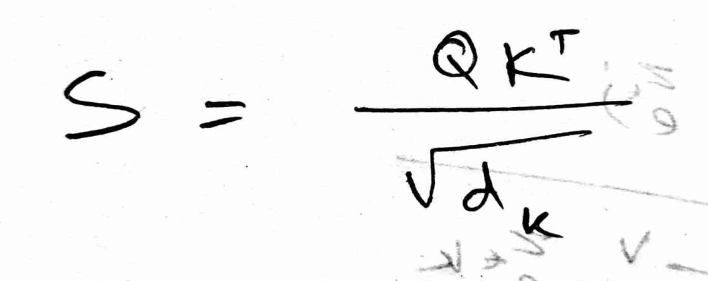
And, in the attention, we add the matrix mask, M:            

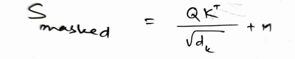
where M can be given as:

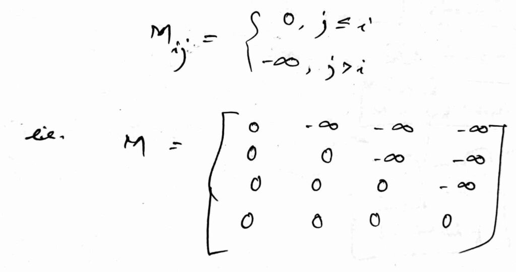
Then, A = softmax(S_masked), and we can say the final output O = AV, where V = value = DW^K.

The Add & Norm is the same as that of the encoder. After masked self-attention, we get

                        D₁ = LN(D + MHA_masked(D, D, D)).

Encoder-Decoder Attention (The Cross Attention)

The attention mechanism here in this part is different. The query, Q, is from the decoder, but the key, K, and value, V, come from the encoder. So, Q = D₁W^Q, K = HW^K, and V = HW^V.

Therefore:

The cross-attention lets the decoder retrieve the relevant information from the input sequence while generating each output token.

Suppose the decoder is currently generating ‘I love … ‘. It needs to determine which source information is relevant for generating the next word. The decoder representation produces a query: q_i. The encoder contains source representations: h₁, h₂, etc. These representations become k₁, k₂, etc. and v₁, v₂, etc. The decoder compares its query against all encoder keys: q_ik₁^T, q_ik₂^T,…, q_ik_n^T. Then, the decoder obtains a context vector: ci, which is given below.

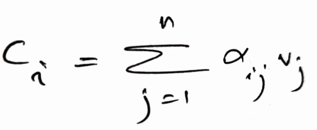
The above paragraph briefly explains the comparison of the decoder query and encoder keys and values.

After cross-attention, the output is sent to Add & Norm. So,

                        D₂ = LN(D₁ + CrossAttention(D₁, H, H)).

Then, D₂ is sent to the decoder Feed Forward Network, i.e., FFN(x) = max(0, xW₁ + b₁)W₂ + b₂. This FFN has the same architecture as that in the encoder, but it has different learned weights. So, F = FFN(D₂). Then, after FFN, Add & Norm is performed again.

Therefore, D₃ = LN(D₂ + F). At this point, one decoder layer is completed, but the decoder has 6 layers, as in the original Transformer, so:

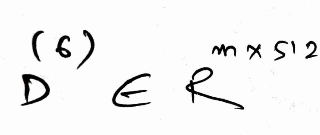
If we are predicting the next token at position t, then the corresponding vector can be given as:

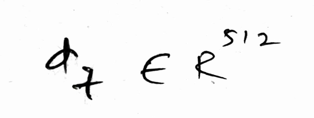
But this dimensional vector isn’t directly a word probability. We need to convert it into a vector whose length equals the vocabulary size.

NB: This linear projection and softmax happen only after all the decoder’s 6 layers are processed. Meaning, each layer is processed up to the FFN, and the Add & Norm component then the output is fed to another layer. After the 6^th layer, the linear projection and softmax are processed.

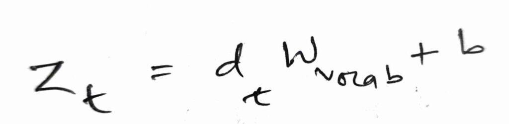
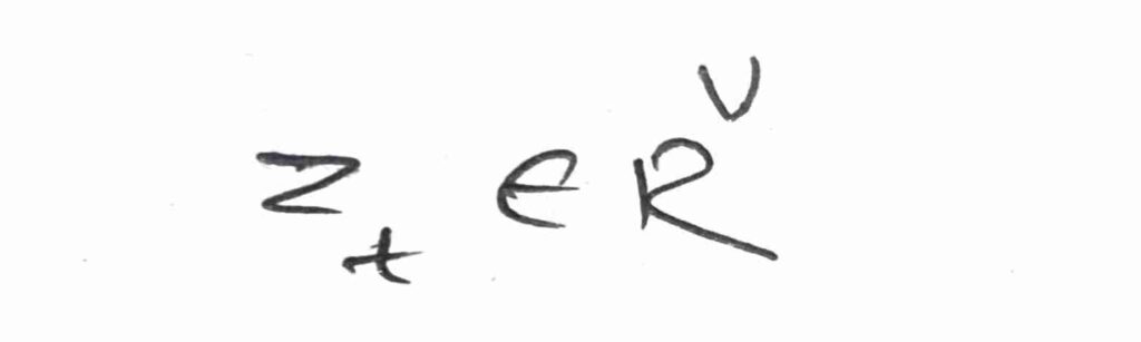
Now we need to perform something called a linear projection to the vocabulary. If V is the vocabulary size, then the output projection matrix is Q. Then the output of the linear projection is given by: z_t. Therefore, z_t in R. This linear projection is used to convert the decoder’s final hidden representation into a score called a logit for every possible vocabulary token. z contains one number, or logit, for every token in the vocabulary, but they are not probabilities yet. So, we apply softmax.

So, if V is the vocabulary size, then the linear projection matrix is given by

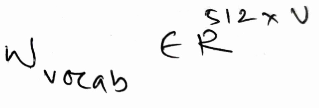
Then, we have output from the linear projection.

where

Then, we apply softmax.

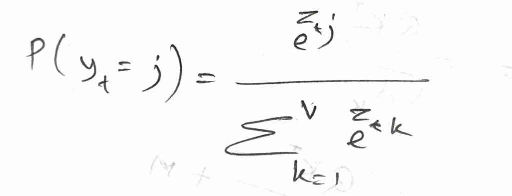
Now, P(y_t = j) is in [0,1], and the sum of the values is 1.

V. TRAINING VS INFERENCE

During training, the source sentence first passes through the encoder, producing the encoder output $H$. At the same time, the correct target sentence is shifted right by one position and given to the decoder. For example, if the target is $[\text{I, am, a, student, EOS}]$, the decoder receives $[\text{BOS, I, am, a, student}]$ and is trained to predict $[\text{I, am, a, student, EOS}]$. This is the teacher-forcing setup: the decoder receives the correct previous tokens rather than its own previous predictions.

The shifted target then passes through all 6 decoder layers. Each layer performs masked self-attention, encoder-decoder cross-attention, and a feed-forward network, with residual connections and LayerNorm. After the sixth layer, we finally have $D^{(6)}$. Only now do we apply the final linear projection and softmax:

$$D^{(6)} \rightarrow \text{Linear} \rightarrow \text{Softmax} \rightarrow \text{probabilities}.$$

These probabilities are compared with the correct target tokens to calculate the loss, and backpropagation updates the model.

During inference, the correct target sentence is unavailable, so there is no teacher forcing. The decoder starts with only $\langle BOS\rangle$, passes it through all 6 decoder layers, then Linear + Softmax predicts the first token. Suppose it predicts I. We then give the decoder $[\langle BOS\rangle,I]$, run it again, and predict the next token. This continues autoregressively:$$\langle BOS\rangle \rightarrow I \rightarrow am \rightarrow a \rightarrow student \rightarrow EOS.$$

So the key difference is simply:

Training: Correct Previous Tokens

Inference: model’s previous predictions​

VI. SOME APPLICATIONS

The Transformer architecture was originally designed for sequence-to-sequence tasks, especially machine translation, but the underlying attention mechanism is now used in many applications.

Machine translation is the original application. For example, the encoder can process an English sentence and the decoder can generate its French, German, or other-language translation. The encoder understands the source sentence, while the decoder generates the translated sentence token by token.

Text summarization is another application. The encoder processes a long document and creates contextual representations. The decoder then generates a shorter summary while using cross-attention to retrieve relevant information from the encoded document.

Question answering can also use encoder-decoder Transformers. The encoder processes a passage and a question, while the decoder can generate an answer based on the information represented in the passage.

Text generation is a major application of the Transformer idea. Decoder-only architectures such as GPT use the decoder’s masked self-attention mechanism to generate text one token at a time. Unlike the original encoder-decoder Transformer, they do not have a separate encoder.

The Transformer architecture was originally designed for sequence-to-sequence tasks, especially machine translation, but the underlying attention mechanism is now used in many applications.

Machine translation is the original application. For example, the encoder can process an English sentence and the decoder can generate its French, German, or other-language translation. The encoder understands the source sentence, while the decoder generates the translated sentence token by token.

Text summarization is another application. The encoder processes a long document and creates contextual representations. The decoder then generates a shorter summary while using cross-attention to retrieve relevant information from the encoded document.

Question answering can also use encoder-decoder Transformers. The encoder processes a passage and a question, while the decoder can generate an answer based on the information represented in the passage.

Text generation is a major application of the Transformer idea. Decoder-only architectures such as GPT use the decoder’s masked self-attention mechanism to generate text one token at a time. Unlike the original encoder-decoder Transformer, they do not have a separate encoder.

VII. CONCLUSION

The encoder-decoder architecture gives one of the best benefits in DL. The Machine translation becomes easy when the encoder-decoder allows seq2seq processing. But there was some limitations – the architecture only processed one token at a time, and even with attention mechanism introduced, the long dependencies of tokens were sometimes missed if the sequence was very long.

So, the Transformer solves this problem by introducing a self-attention mechanism. The self-attention mechanism is nothing but a mechanism to capture the valuable relationships between tokens. It gives contextual understanding of the token itself and surrounding tokens. Then, again in the decoder, the masked multi-head attention uses a technique of masking the future tokens. This forces the decoder to look for the future token. Then the cross-attention uses both the encoder’s output and the output from the masked multi-head attention, and this allows it to have the relevant information from the input sequence while generating each output token.

References

Vaswani, A., Shazeer, N., Parmar, N., Uszkoreit, J., Jones, L., Gomez, A. N., Kaiser, L., & Polosukhin, I. (2017). Attention is all you need. Advances in Neural Information Processing Systems, 30, 5998–6008.

• YouTube
• Facebook