


The article is succeeded article of The Transformer. T5 is a model that can perform many NLP tasks. In this article, we didn’t show how to use T5 with code; however, we will update and to not miss updates, please subscribe to our Newsletter.
List of content:
- Introduction
- T5
- Pre-training
- Fine-tuning
- Inference
- Conclusion
- Reference(s)
I. INTRODUCTION
Natural Language Processing (NLP) is a branch of Artificial Intelligence (AI). It deals with natural language. Or, we can say, it is the step-by-step process of operations we perform on natural language to let machines understand, process, and respond. When we speak English, some people can understand what we are talking about, but some can’t if they don’t understand English. The same problem exists with other languages. So, we need NLP.
In 2017, the Transformer architecture was introduced and made everyone rethink how they think about AI, especially in NLP and Gen AI. In 2020, Raffel, C. et al. introduced something valuable to the world. The Transformer is based on the encoder-decoder architecture, and it’s best suited for machine translation. But Raffel and other researchers thought that we could have a general-purpose model based on the Transformer that can perform many NLP tasks, such as machine translation, summarization, etc.
The T5, Text-to-Text Transfer Transformer, was introduced by Raffel, C. et al. in their paper, “Exploring the Limits of Transfer Learning with a Unified Text-to-Text Transformer”. The basic idea of T5 is that it takes text as input and produces text as output. The best question they asked themselves was, “Can the same model solve translation, summarization, question answering, classification, and other NLP tasks if every task is represented as text going in and text going out?” This is the foundation of T5.
II. T5: Text-to-Text Transfer Transformer
The transformer is based on the encoder-decoder idea; the encoder reads the source sentence and the decoder generates the translated sentence. Based on this idea, T5 was introduced, but T5 is a general-purpose pretrained model for NLP. So, it keeps the Transformer idea but uses the concept that if a model is trained on a vast amount of text data, we can use this model to perform many NLP tasks. It treats every task as a text-to-text task; that’s why the name is Text-to-Text Transfer Transformer.
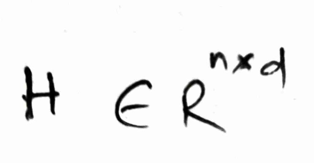
T5 is still an encoder-decoder Transformer at the architectural level. Suppose the input sequence is X; X is tokenized and converted into embeddings. These representations are passed through the T5 encoder and self-attention, and then produce the encoder output H (please read the article, Rise of the Modern AI Empire – The Transformer, for basic understanding).
Conceptually, X -> Encoder -> H. Then the decoder receives the target side information and uses two types of attention. First, it performs masked self-attention, and second, it performs cross-attention. The pipeline of T5 can be given as:
Input -> Encoder -> Cross-Attention -> Decoder -> Vocabulary probabilities
T5 is not simply the encoder and decoder. It is pretrained, meaning T5 is trained first and used for a particular task, not input-train-output; T5 uses the transfer learning idea. T5 uses pre-training and then fine-tuning. During pre-training, T5 receives enormous amounts of ordinary text without requiring human-provided task labels. It learns general language patterns by solving a reconstruction problem. After this, for a particular task like translation or summarization, the model can be fine-tuned.
III. PRE-TRAINING
Before we use T5, it undergoes training with enormous text data. During this, T5 learns general patterns of language; the purpose of pre-training is not specifically to teach the model translation, summarization, or question answering but to learn the patterns.
In pre-training, there is an interesting idea that was used in this model. We call this span corruption. Suppose “The cat is sleeping on the mat” is the sentence. T5 corrupts part of the sentence. The sentence becomes “The cat <extra_id_0> on the mat”, and the missing span is “is sleeping”. Then the model is trained to generate: < extra_id_0> is sleeping <extra_id_1>. This forces the model to learn the patterns, relationships, etc. about the text. The span corruption happens after tokenization but before embedding (first I want you to know this idea, because tokenization and embedding are to be shortened).
The T5 models use SentencePiece for tokenization and assign token IDs. These IDs are converted into embeddings. Then, the embeddings are fed to the encoder. At this time, T5 doesn’t use the Positional Encoding from the original Transformer; it uses the position bias that gets added during attention.
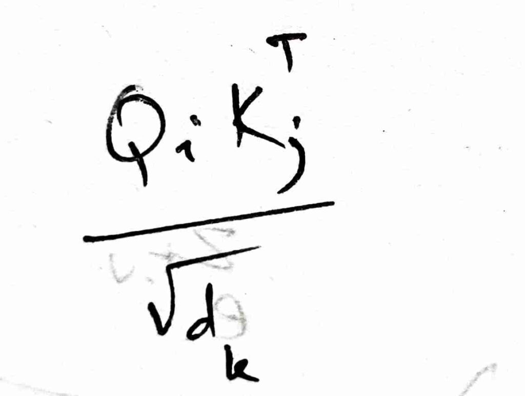
For one attention head, the attention score between query position i and key position j is based on:
T5 modifies this by adding the position bias:
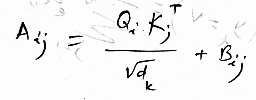
where Q = XWQ, K = XWK, V = XWV, and Bij is the position bias associated with the distance between positions i and j.
So, the attention is given by:
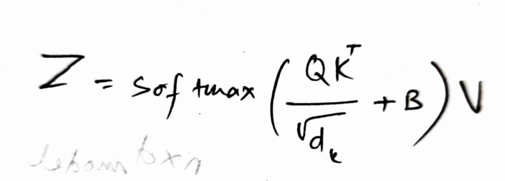
The bias B tells the attention about the relative location of tokens without adding a sinusoidal positional vector to every token embedding. Here, a little modification: T5 uses pre-normalization before attention, meaning that before normalization it uses RMSNorm instead of the standard LayerNorm.
NB: the symbols or representations are used to make the idea easier compared to the original Transformer.
The attention score is calculated for heads (heads are different in number) and then concatenated:
O = Concate(Z1, Z2, …, ), where Z represents the attention scores of the heads.
Then projected: Oproj = OWo
Now, T5 applies Dropout and a residual connection:
O’ = Dropout(Oproj)
Then, the original input (if H0 is the one) is added: H1 = H0 + O’.
This is the residual connection, and we can represent the flow up to this by the formula below.
H1 = H0 + Dropout(SelfAttention(RMSNorm(H0)))
Again, before the Feed Forward Network, we have normalization: RMSNorm.
NB: In this part, the formula for RMSNorm.
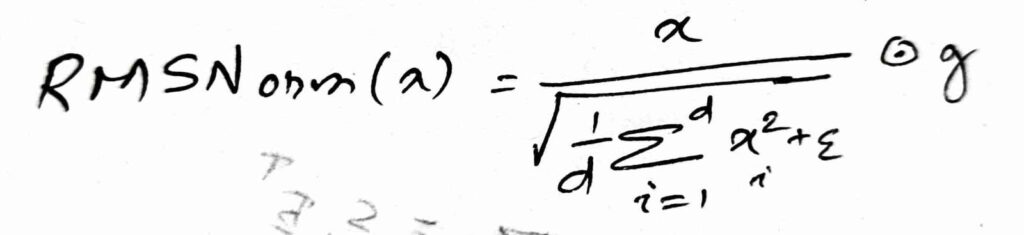
where x= input vector, d = dimension, xi = each element of x, ε = small value for numerical stability, g = learned scaling parameter, and ⊙ = element-wise multiplication.
So, Hr = RMSNorm(H1).
Then, it goes to the FFN. So, DenseReluDense(x) = W2ReLU(W1x + b1) + b2. However, T5 implementations/configurations can use a gated activation such as GELU/GEGLU-style variants, so the exact FFN form depends on the T5 variant/configuration. The original formulation is given below.
F = W2ReLU(W1Hr).
The FFN is applied to every position independently, because the self-attention layer mixes information between tokens. After the FFN, there is another Dropout and a residual connection (RMSNorm). F’ = Dropout(F). Then, H2 = H1 + F’; H2 is the output of the first encoder, and the steps are repeated for all the encoder layers.
Therefore, if all the encoder block completes, we can say: H = Encoder(X), where
On the decoder side, the target input is span-corrupted and then embeddings, but the decoder input is always right-shifted. Let’s change the example here: if our sentence is “I love you”. In the encoder (for example), the span-corrupted one is “I <extra_id_0> you,” but in the decoder’s input, the sentence becomes “<extra_id_0> love <extra_id_1>” after span corruption. And then, the right-shifted one will be (conceptually) “<pad> <extra_id_0> love <extra_id_1>” while the labels are: <extra_id_0> love <extra_id_1> <eos>”.
Then, the decoder input tokens are converted into embeddings using a shared embedding matrix. Then, masked self-attention is performed. Say, in the input above, <extra_id_0> will see only itself and previous information (if any), and <extra_id_1> will see only itself and previous information, for example.
The formula for masked self-attention is given by adding another matrix called M (masked).
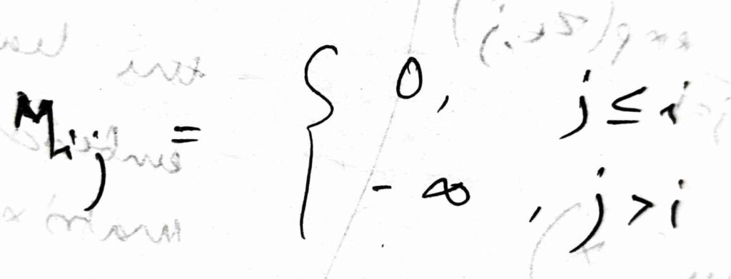
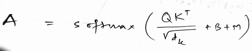
The negative infinity ensures that future positions receive probability zero.
So, the first sublayer follows: D1 = D0 + Dropout(SelfAttention (RMSNorm(D0)), where RMSNorm is performed before attention.
Then, the cross-attention happens here. The decoder needs information from the encoder now. The decoder representation becomes the query. Q = DnormWQ. But the keys and values come from the encoder output: K = HWK and V = HWV.
The decoder computes:
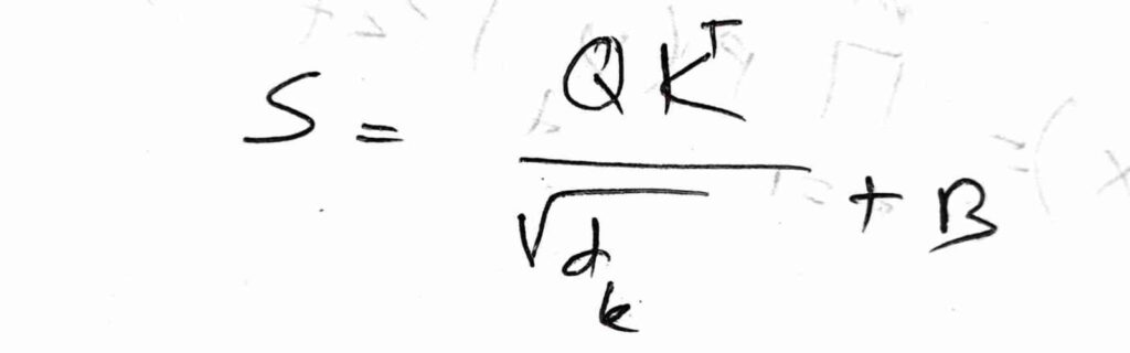
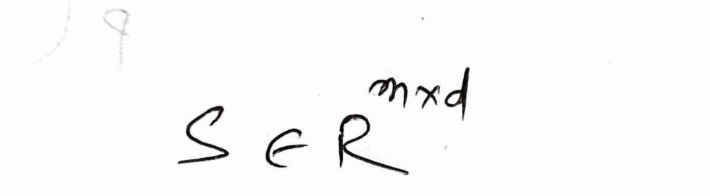
And A = softmax(S), then the output becomes O = AV.
So, D2 = D1 + Dropout(CrossAttention(RMSNorm(D1), H).
Then, the decoder FFN: Df = RMSNorm(D2), then FD = FFN(Df).
Again, there is dropout and a residual connection: D3 = D2 + Dropout(FD). This is repeated for all decoder layers.
The final decoder representation is: S = Decoder(Yshifted, H), where S = 0 (after all the layers are done).
Now, T5 uses the shared embedding matrix for the vocabulary projection. For a decoder hidden state st: zt = stET, where
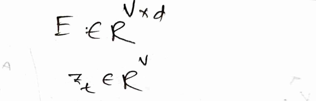
These are the logits for every vocabulary token. So, the logits become probabilities:
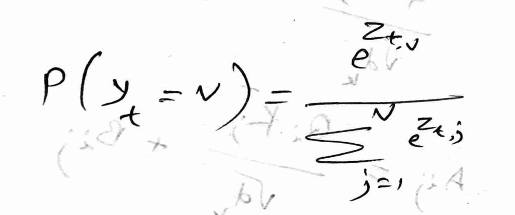
After this, we have cross-entropy loss and backpropagation, then update the T5 parameters. The complete computation pipeline is shown in the picture below.
Now we have the very important parts of T5. Fine-tuning and Inference. Pre-training teaches T5 general language understanding using span corruption. Fine-tuning teaches T5 how to perform a specific task. Inference is when we actually use that task-specific model.
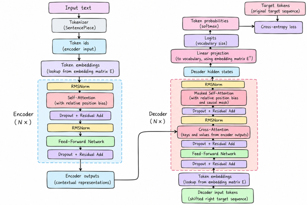
Fig. 1: T5 Pre-training diagram.
IV. FINE-TUNING
After T5 has completed pre-training, it has learned general language representations and sequence generation through span corruption (in the paper, the span corruption objective). However, the pre-training task is not necessarily the task we ultimately want the model to perform. For example, if we want T5 to perform translation, summarization, question answering, or classification, we need to adapt the pretrained model to that particular task. This process is called fine-tuning. The important idea behind T5 is that these different NLP tasks are all converted into the same text-to-text format. Instead of creating a separate classification head, translation head, or summarization head, we give T5 a textual input and train it to generate a textual output.
For example, for summarization, a training example can conceptually be represented as an input sequence containing an instruction such as summarize: followed by the document, while the target sequence contains the desired summary. For translation, the input could contain translate English to German: followed by the English sentence, while the target contains the German translation. So, during fine-tuning, instead of constructing a corrupted input and asking the decoder to reconstruct missing spans, we provide the actual task input X and the desired task output Y.
Using SentencePiece, both the input and target output are tokenized.
X = [x1, x2,…,xn] and Y = [y1, y2,…,ym].
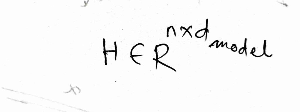
The input token IDs are converted into embeddings, then passed through the stack of T5 encoder blocks. The encoder performs its normal computations – RMSNorm, self-attention, etc. Then, the final result is a sequence of contextual representations and can be written as:
H = Encoder(X), where
Unlike pre-training, there is no span corruption here. The encoder receives the actual input required by the downstream task.
The decoder is then trained to produce the target sequence, Y. During training, T5 uses teacher forcing. The target sequence is shifted to the right, so the encoder receives something conceptually like [<start>, y1, y2,…,ym-1] and is trained to predict [y1, y2,…,ym, <eos>].
At every decoder position, the decoder first performs masked self-attention. The causal mask prevents a position from accessing future target tokens. Therefore, when the model is learning to predict yt, it can use y1,…,yt-1, but not yt+1, yt+2,… The decoder then performs cross-attention against the encoder output H. In this cross-attention, the decoder representation provides the queries, while the encoder representations provide the keys and values. This allows the decoder to combine the information it has already received from the target side with information contained in the original input.
After passing through the decoder’s layers, each target position has a decoder hidden state st. T5 then maps this hidden state into the vocabulary space. Using the shared vocabulary embedding matrix, the logits can be represented as:
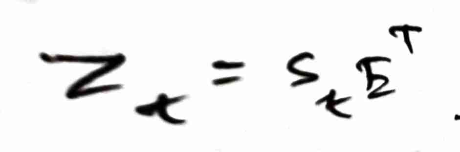
where E is the learned embedding matrix of T5.
The resulting vector contains one logit for every token in the vocabulary. Softmax converts these logits into probabilities:
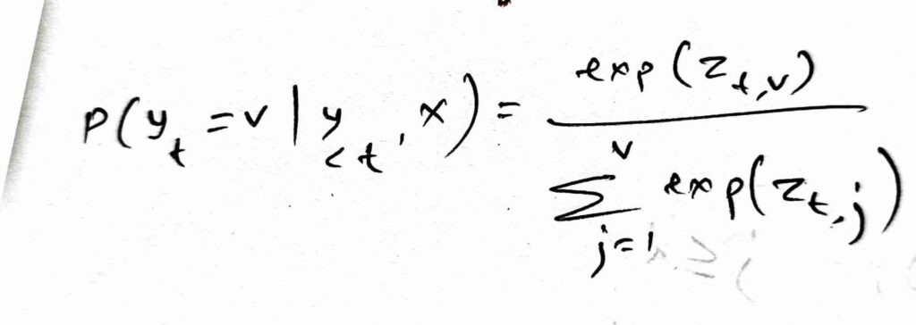
The probability assigned to the correct target token is then used to calculate the cross-entropy loss. For the complete target sequence, the autoregressive loss is given below.
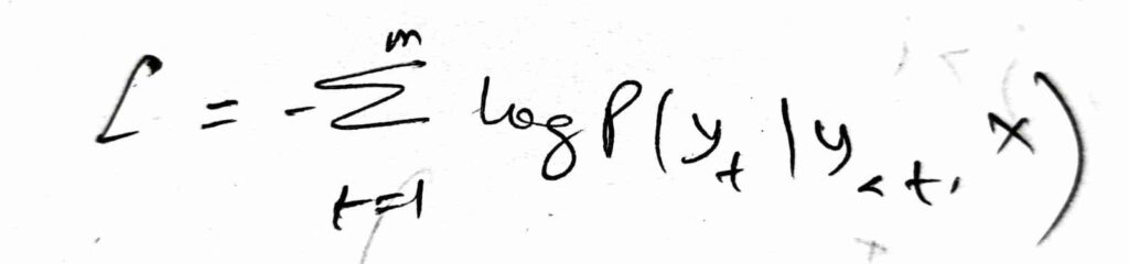
The loss is backpropagated through the decoder, cross-attention, encoder, and the rest of the network. The parameters are then updated using gradient descent or an optimizer such as Adam. Repeating this over many task-specific examples causes the pretrained T5 parameters to adapt from general language modeling knowledge toward the particular task.
The important distinction from pre-training is therefore the source of the target. During pre-training, the target consists of spans removed from the original text. During fine-tuning, the target is the desired output of a particular task. The underlying encoder-decoder computation is still T5, but the model is now learning P(Y | X), for the particular task represented by the fine-tuning dataset.
V. INFERENCE WITH T5
Once fine-tuning is complete, we can use the resulting model on an input it has never seen during training. This is called inference. The biggest difference between fine-tuning and inference is that during fine-tuning we know the correct target sequence, whereas during inference we do not. Therefore, the model has to generate the target itself.
The input here is also tokenized, then converted into embeddings and passed through the entire encoder, and produces its contextual representation, H. At this point, the encoder has finished processing the input. Unlike fine-tuning, there is no correct target sequence available, so the decoder now has to generate the output. So, the generation begins with the decoder’s starting token. The decoder processes this initial input while attending to the encoder representations through cross-attention. After passing through the decoder layers, the decoder produces a hidden state s1 for the first output position. T5 projects this hidden state into the vocabulary space: z1 = s1ET.
Softmax then produces a probability distribution: P(y1 = v | X). The model now has a probability for every possible vocabulary token. For example, one token may have a probability of , another , another , and so on. The model must now use a decoding strategy to select the next token. With greedy decoding, the token with the largest probability is selected: y1 = argmaxv P(v|X).
Other decoding strategies can also be used, such as beam search or sampling, depending on the application and generation configuration.
Once the first token has been selected, it is fed back into the decoder as part of the decoder’s input. The decoder now has the beginning of its own generated sequence and calculates the next probability distribution: P(y2 | y1, X). The second token is selected, appended to the sequence, and fed back again. The process therefore becomes autoregressive: P(y1 | X), then P(y2 | y1, X), then P(y3 | y1, y2, X) and so on. And in general, we can express it as like the below one.
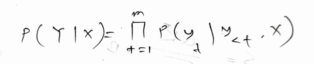
This loop continues until the model generates an end-of-sequence token, usually represented as <eos>, or until the configured maximum output length is reached. The sequence of generated tokens is then decoded back into text by the tokenizer.
In inference, most of the time, there is no loss calculation or backpropagation. Meaning the parameters of the model are frozen, we simply perform forward passes through the encoder and decoder and use the resulting probability distributions to generate the output.
VI. CONCLUSION
T5 is an NLP model that treats every task as a text-to-text problem. The main idea behind T5 is that one model for many NLP tasks. Meaning, a model is trained on a very large amount of text, and the model can be used for many tasks like machine translation, summarization, question answering, etc.
The architecture is equivalent to the original Transformer. T5 also uses an encoder-decoder, self-attention mechanism, cross-attention, etc. But T5 uses RMSNorm before attention as one of the differences. Another one is that T5 uses SentencePiece tokenizer and some positional bias for positions. We can fine-tune T5 for a specific task. Also, we can use T5 for inference.
NB: Inference of T5 for summarization will be updated on our official site and also on our official YouTube channel.
REFERENCES
Raffel, C., Shazeer, N., Roberts, A., Lee, K., Narang, S., Matena, M., Zhou, Y., Li, W., & Liu, P. J. (2020). Exploring the limits of transfer learning with a unified text-to-text transformer. Journal of Machine Learning Research, 21(140), 1–67.
Vaswani, A., Shazeer, N., Parmar, N., Uszkoreit, J., Jones, L., Gomez, A. N., Kaiser, Ł., & Polosukhin, I. (2017). Attention is all you need. Advances in Neural Information Processing Systems, 30, 5998–6008.