


- INTRODUCTION
- NEURAL MACHINE TRANSLATION
- ATTENTION MECHANISM
- CONCLUSION
I. INTRODUCTION
We booked a ticket to China. When we land in China, we will first try to book a cab to our hotel. Or, forget about landing and booking a cab. Once we are in China, we will go to dinner or lunch. However, how are we going to order? We need to know and understand Chinese, right? Or do we bring a translator? All these answers depend on us. So, if we are visiting China alone, we need some way of translation. China is one of the fastest-developing countries in the world of Artificial Intelligence. We can use an application for translation.
China has built many translators, from English to Chinese language for example. When we visit China, we should make sure that we have installed a translation application, from our language to Chinese or from English to Chinese. So, when we say translation, one thought that comes to our minds is that it needs a human being to translate the languages. Yes, we need human beings for this. However, we can use a translator with just our smartphones.
The translation using our smartphones or a machine is called Machine Translation (MT). The working of MT using the Attention Mechanism and Self-Attention Mechanism will be available in the project submenu in the coming days.
II. NEURAL MACHINE TRANSLATION
We can set some rules for a task. For example, when we are preparing tea, we need to add a full tablespoon of sugar and two full tablespoons of milk powder. This is our rule. For someone, this will be different. So, for a task, we can use or set some rules to accomplish it. These systems or these tasks are called rule-based systems or rule-based tasks. Approximately 70 years ago, translation was a rule-based system. Every grammatical form, word meaning, etc., was handwritten. Then, Statistical Machine Translation (SMT) evolved. In SMT, translation is treated as a search for the target sentence that maximizes the combined probability of two separately learned statistical models – a translation model, learned from large parallel corpora via statistical word/phrase alignment, which estimates how likely a given source phrase corresponds to a given target phrase; and a language model, learned from large monolingual target language text, which estimates how fluent or natural a candidate target sentence is. A decoder then searches over possible translations to find the one that best balances faithfulness to the source with fluency, rather than translating word-for-word or relying on handwritten rules. We know that MT is a translation system using a machine. Neural Machine Translation (NMT) is a translation system that uses neural networks. NMT became popular with Deep Learning techniques. We can also say that NMT uses Deep Neural Networks to translate. In NMT, an encoder reads the source sentence and converts it into contextual vector representations that capture the meaning and relationships between words. A decoder then generates the target sentence one word or one token at a time. This was done, surprisingly, using the Attention Mechanism (which is explained in the next section) and, nowadays, the Self-Attention Mechanism is used.
III. ATTENTION MECHANISM
When we teach our children the first lesson, we tell them to pay attention. What does that mean? That means the real focus they should have on the lesson they are reading, with full consciousness and emotion. However, in AI, when we talk about attention, it is not human attention. Human attention and the attention mechanism (even the self-attention mechanism) are different from each other. The attention mechanism is based on numbers that are calculated from a mathematical formula using data weights for relationships. However, human attention is very different from this. Human attention is based on focus, emotion, and even goals, so it can filter the inputs so easily.
The attention mechanism we are going to understand here is based on the attention mechanism that was presented by Bahdanau et al. in 2015 (first preprint in 2014) in the paper “Neural Machine Translation By Jointly Learning To Align and Translate”.
The encoder-decoder architecture we discussed in the previous article is the base architecture for Machine Translation. Even though the architecture does the job efficiently. Bahdanau found a flaw or bottleneck in the architecture. The encoder-decoder processes a variable-length source sentence or input into a fixed-length context vector. This works for short sentences very well, but when the sentence is too long, it misses context relationship. Bahdanau proposed the attention mechanism to solve this bottleneck.
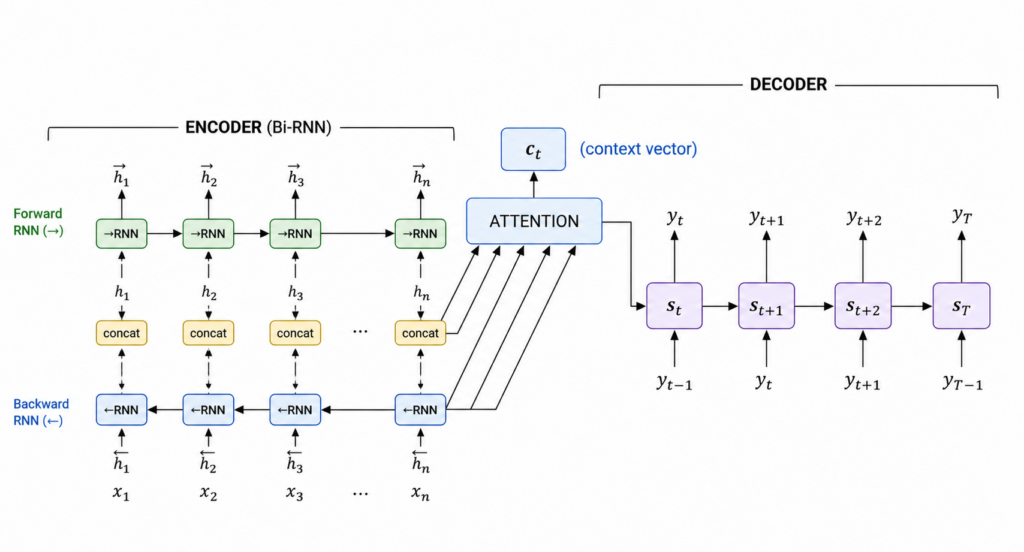
Fig. No. 1: Attention Mechanism
We can ask ourselves, “What information should the decoder use from the source sentence when generating each token or word?” We can say that this question is the basic idea in the Bahdanau et al. paper. The authors don’t change the architecture of the encoder-decoder, but they just change the workflow.
Bahdanau et al. use a bidirectional RNN as the encoder. For two RNNs, there will be separate groups of hidden states. So, we have a forward RNN and a backward RNN (bidirectional RNN). Let’s denote the hidden states of the forward RNN as F and those of the backward RNN as B (the paper has its own notation, but in this article let’s simply change the notations to not to get confused). Suppose we have a source sentence like x = (x1, x2, x3, …, xTx). For this input position denoted as j, the encoder produces information hj. Mathematically, we can represent this as:
hj =[F/B]
So, the encoder produces h1, h2, h3, …, hTx. These are called annotations in the paper. These annotations have source position and information from surrounding.
In the paper, we don’t focus on the encoder part. We focus on the decoder because the attention mechanism is on the decoder side. And in this article, we use a simple explanation of the attention mechanism.
The annotations are generated or produced by the encoder, but the decoder doesn’t look at them all at first. Because if the decoder uses all the annotations, the model won’t know the information about the source sentence positions that are relevant to the current target word. For every decoding step i, the decoder has si-1 as the previous state. The decoder also has the annotations: h1, h2, … hTx from the encoder. The attention happens here. The decoder compares si-1 with the annotations hj. For every source position j, it computes an alignment score: eij = α(si-1, hj), where α(si-1, hj) = vaTtanh(Wasi-1 + Uahj), where Wa and Ua are weight matrices as Wa ∈ ℝn′×n and Ua ∈ ℝn′×2n, n = decoder hidden-state size and n′ is the hidden size of the alignment network (according to the paper). The paper defines eij as a score indicating how well the source information around position j matches the decoder’s current state for generating target word yi. The alignment score can also be called additive attention, as the decoder state and encoder annotation are added before the nonlinear transformation.
However, the alignment scores are not attention yet. The alignment scores are converted into attention weights with the formula:
αij = exp(eij)/∑Tx exp(eik). (The paper explicitly interprets αij as the probability that target word yi is aligned with source word xj).
Suppose we have αij = [0.5, 0.1, 0.001, 0.60, 0.70]. The model says position 5 is more important, but positions 1 and 4 contribute. This is the soft alignment in the paper.
Again, the context vector is calculated using the annotations hj and the attention weights, αij. Mathematically, the paper presents the context vector as ci.
ci = ∑Tx αijhj, the context vector for the decoding step i.
Then, the context vector is fed to the decoder for the next decoding step. The whole process is repeated again and again until a special token is met. This is the key reason it is called dynamic attention.
So, one clarification we like to mention from the paper is that si-1 is the previous state of the decoder at step i. But the decoder uses an initial state as s0 = tanh(WsB1). Ws is also a weight matrix, but it is from the encoder side, where Ws ∈ ℝn×n . The initial state of the decoder doesn’t know anything about the target sentence, so s0 is initialized from the encoder and provides the decoder with an initial representation derived from the source sentence.
IV. CONCLUSION
The encoder-decoder architecture is the architecture that maximizes the efficiency of Machine Translation. In 2014, Machine Translation started with Neural Machine Translation. The encoder encodes the source sentence into a fixed-length vector, and the decoder tries to decode everything from this fixed-length vector. This works well for short sentences, but it lacks contextual relationships in long sentences.
After some months in 2014 (first preprint, but officially in 2015), Bahdanau et al. introduced an idea for solving this problem. On the encoder side, annotations are produced. Using the annotations, the decoder produces alignment scores and attention weights. The attention weights are then used with the annotations to produce the context vectors of each generation step. We can say that the authors allow the decoder to use all the annotations from the encoder side to get more contextual information about a source sentence. This is the attention mechanism Bahdanau et al. introduced.
REFERENCES
Bahdanau, D., Cho, K., & Bengio, Y. (2014). Neural machine translation by jointly learning to align and translate (arXiv:1409.0473). arXiv. https://doi.org/10.48550/arXiv.1409.0473
Sutskever, I., Vinyals, O., & Le, Q. V. (2014). Sequence to sequence learning with neural networks (arXiv:1409.3215). arXiv. https://doi.org/10.48550/arXiv.1409.3215